Artificial Intelligence Pyramid
Artificial Intelligence (AI) evolution can be categorized into four levels based on depth of intelligence.
- Symbolic AI (Business Intelligence)
- Statistical Analysis and Optimization
- Machine Learning
- Deep Learning
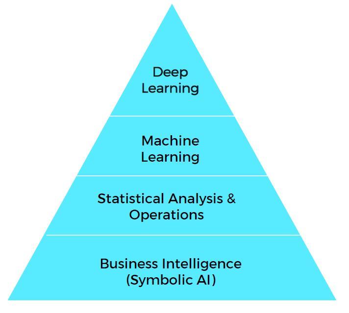
Artificial Intelligence Pyramid
Symbolic AI
This is rule-based intelligence, similar to classical programming. It has an element of intelligence or decision support, but there is no learning element. An example is, once the quantity of a product in a retail store goes below a certain threshold, an order for a specified quantity, is automatically placed to a warehouse or supplier. This is also known as Business Intelligence (BI) in the industry. This itself has many layers of intelligence starting with historic MIS (Management Information System/ descriptive analytics), OLAP (pivoting, drill down/up/through, what-if analysis or diagnostic analytics), self-service BI etc. Cognos (acquired by IBM), Business Objects (acquired by SAP), MicroStrategy, Microsoft SSRS/SSAS, and Oracle Express/OBIEE were the early entrants in this area, which is now being dominated by Tableau, QlikView and Microsoft PowerBI.
Statistical Analysis and Optimization
Statistics is a branch of mathematics that deals with the analysis of data to understand its distribution and make inferences on population parameters such as mean, variance with certain confidence level. It laid the foundation for today’s machine learning.
The objective of this analysis is to understand patterns in the data and relationships among various attributes that enable prediction and classification.
Statistical analysis typically uses very small sample data for the analysis and prediction. Most of the techniques involve comparison of intra and inter group variance based on a hypothesis. Statistical analysis also includes regression and discriminant analysis, but they use analytical methods (e.g. solving linear equations directly) as opposed to numerical methods (which are used in Machine Learning and Deep Learning). Hence, there is no learning involved in these methods.
Statistical analysis makes lot of assumptions on input data as well as in the predictions they make, which is a limitation of these techniques.
Following are the various tools, methods and algorithms used in statistical analysis
- Introduction to Statistics
- Descriptive Statistics
- Graphs and Charts
- Probability Theory
- Distributions and Sampling
- Making inferences about population parameters
- Simulation
- Optimization
- Factor Analysis
- Regression and Time Series Analysis (forecasting numerical variable)
- Discriminant Analysis (classification)
- Conjoint Analysis
- Cluster Analysis
- Market Basket Analysis (Apriori and Association Rules)
Machine Learning
Machine Learning (ML) is the natural extension of statistical analysis. It deals with more complex problems and with enterprise scale data. It is also called Data Mining in the enterprise world.
These algorithms use numerical methods that are iterative in nature during the training to minimize the error (optimization) and update model parameters (weights/biases) that is called as learning.
Following are the two formal definitions of machine learning :
Machine Learning: A field of study that gives computers the ability to learn without being explicitly programmed.
- Arthur Samuel (1959)
Arthur Samuel coined the term “Machine Learning” in 1959!
Well-posed Learning Problem: A computer program is said to learn from experience E with respect to some task T and some performance measure P, if its performance on T, as measured by P, improves with experience E.
- Tom Mitchell (1998)
Popular Machine Learning Algorithms
There is a large number of ML algorithms that have been developed over the years in various fields such as Operations Research, Statistics, Econometrics, Data Mining using different approaches, all of which are now coming under the larger ML umbrella. Given below are the broad categories of algorithms and sample algorithms within each of those categories:
- Discriminative Algorithms (Linear Regression, Logistic Regression)
- Generative/Probabilistic Algorithms (GaussianNB, MultinomialNB, BernoulliNB, LDA, QDA)
- Kernel Methods (Support Vector Machines)
- Matrix Decomposition (Eigen Decomposition, Singular Value Decomposition)
- Time Series (ARIMA, Holt-Winter algorithms)
- Shallow Neural Networks
- Recommendation Systems/Engines(Surprise)
- Non-parametric (K-nearest neighbor/KNN)
- Ensemble Methods
- Bagging (Decision Trees, Random Forests)
- Boosting (Adaboost, Gradient Boosting)
- Stacking (mlxtend, XGBoost)
How do ML Algorithms work?
All these algorithms typically form an internal representation of data that maps input data to the desired output. To give an idea on how this representation looks, we will examine Linear Regression and Logistics Regression Algorithms in detail below. These are the earliest algorithms developed much before the ML and Statistical Analysis fields emerged. They are like grandparents of today’s machine learning!
Linear Regression
Regression Analysis is a method for finding the relationships/associations between variables. Linear regression deals with the linear relationship between variables. If the dependent variable is Y, and independent variables are X1, X2, X3 etc., then the relationship among them takes the form as given below
Y = a0 + a1*X1 + a2*X2 + a3*X3 + …, where a1, a2, a3 are the coefficients of X1, X2, X3 independent variables and a0 is the constant that accounts for any unknown/unmeasurable independent variables other than known variables X1, X2, and X3.
With the training data set, these algorithms find values for all coefficients a1, a2, a3 and the constant a0. Once we have this full equation, then for any future values of X1, X2, X3, we can predict Y! The process of finding these coefficients is called training/learning. This is an iterative process of predicting Y, measure the error between predicted Y and actual Y (from historic training data), using which update coefficients, and this process goes on till the error is minimized to the lowest possible value.
In statistical analysis, the same problem is solved in one shot, without iterations, using an analytical solution that requires the computation of matrix inverse. In statistical analysis, training examples are small (as we take only sample data), and number of variables is very less, so it is computationally possible to compute matrix inverse and get an analytical solution which is guaranteed to provide best solution.
In Machine Learning, data volume is large (as we take population data), and the number of variables is also very large., More importantly, we remove the assumption that these independent variables have no correlation among them. When there is a strong correlation among these variables, computation of matrix inverse may not be possible. Also, the volume of data and large number of variables make it highly time consuming, if not impossible to compute. Hence, we go for a numerical solution using optimization algorithm. Numerical methods have a risk of getting stuck in local minimum, instead of global minimum (best possible solution), hence, may result in sub-optimal solution.
- Simple Linear Regression: This involves only one independent variable so the equation takes the form of Y = a1*X1 + Constant.
- Multiple Linear Regression: Here we have more than one independent variable.
- Time Series Regression with seasonality and trend factors: Here the independent variable is the time, e.g. prediction of stock prices, inflation, GDP growth etc. over a time period.
Logistic Regression
This is similar to linear regression, but the dependent variable Y is categorical and binary (can take 0 or 1 only). It is a classification algorithm used to assess if a person defaults on the loan or not, if a customer moves away from the service or not (churn), if a particular claim is a fraudulent or not etc.
The relationship between dependent variable and independent variables is determined by estimating the probabilities using a logarithmic function. Ln(p/(1-p)) = a0 + a1*X1 + a2*X2 + a3*X3 ….+ an*Xn
Using historical data, the coefficients a0 to an are estimated. Then the model is ready to classify the dependent variable for any given set of independent variable values.
It can also be used in multi-class problems, e.g. classifying a hand-written digit into 0 to 9, one of the 10 classes.
This algorithm also uses numerical optimization methods to compute coefficients.
As can be seen from the way these algorithms work, they are essentially mapping input to output through an equation. This equation can also take nonlinear polynomial terms.
Other ML Methods
Probabilistic algorithms use probability distributions like Gaussian, Bernoulli for mapping input to output, instead of an equation.
Kernel Methods use higher dimensional representation of original training data to map input to output.
Neural Networks use its parameters (weights and biases in each of the layers) to map input to output.
Non-parametric models don’t have any learning process, hence, no parameters to learn. They simply compute geometric distance between various observations in the training data, and map unknown observations to the class of nearest known observations.
Essentially, they all use different approaches to map input to output, by forming an intermediate representation of original training data that clearly separates various classes of observations.
Deep Learning
As we have seen, many different algorithms (statistical and machine learning) have been developed for solving various problems over a period of time. Motivated by how the human brain is able to handle varieties of problems, researchers started looking for a general-purpose algorithm that can solve many different problems. The same motivation earlier had resulted in today’s massive computing platforms that can handle wide variety of problems at large scale, as opposed to having different devices such as calculators, alarm clocks, music/video players, phone etc.
The result of those efforts is Artificial Neural Networks (ANNs). The same on/off logic gates that formed massive computing platforms, form the basic building blocks of neural networks. This micro unit is called perceptron or neuron.
ANNs try to mimic the way the human brain works. Our brains consist of billions of neurons connected with one another, and the strength of each of these connections relate to various functions of the brain. Similarly, ANNs are modeled with multiple layers of neurons, with one input layer, one output layer and one or more hidden layers in between as shown below.
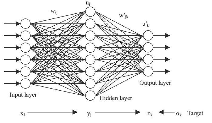
Artificial Neural Networks
At each of the nodes (neuron), the following computation takes place to arrive at an output that the node sends to other nodes connected with it in the next layer.
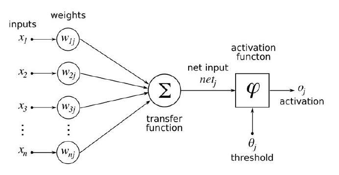
ANN Computation
There are many types of neurons based on their activations (binary threshold, linear, sigmoid etc.), and many types of neural networks based on their architecture (Dense, CNN, RNN etc.). There are several different cost equations used to optimize the network.
The name Deep Learning (DL) comes from the fact that these networks can have many hidden layers, and the deeper the network the more complex problem it can solve. It also differs from ML in that it requires careful hand crafting of features that influence the target variable. DL does not require any feature engineering, and the algorithm discovers by itself which features are to be used. For example, to predict the price of a house, in ML, we will have to manually pick up variables that have higher influence on the price of the house from an exhaustive list of over 150 variables that describe a house. At times we may have to create different sets of attributes from directly observed attributes. In DL, we just need to pass on all observed attributes that describe the house and algorithm will pick up that ones that are most relevant for the problem.
Given the layered architecture it learns hidden patterns in the data hierarchically. That means each layer abstracts the features at a higher level compared to the previous layer. In the example of image processing, the first hidden layer after image input, tries to identify low level features like edges, corners etc., then the next layer tries to combine some of these edges to form simple shapes, and subsequent layers continue to build on them all the way to detecting and localizing all the objects in the picture towards the end of the network, closer to output.
Though their fundamental building blocks are the same, different architectures have been developed to solve different type of problems with different types of data. Following are a few popular neural networks.
Feed Forward/Dense Neural Networks (Dense)
In this type of network signals pass only in one direction, from input to output layers. No backward or sideways connections exist. Every neuron in one layer is connected to every other neuron in the subsequent layer, hence, they are called Dense Networks. In early days only one hidden layer was used, in between input and output layers. Hence, these were also called shallow neural networks.
Though this type of network can solve many ML problems, it can’t handle computer vision, speech recognition, or NLP kind of applications, as they involve dependencies in the input data sequence, or pixel positions in the image.
This was the architecture used before arrival of Deep Learning.
Recurrent Neural Networks
The idea behind Recurrent Neural Networks (RNN) is to make use of sequential information. In a traditional neural network, we assume that all input variables (and outputs) are independent of each other. But for many tasks that assumption does not hold good. If we want to predict the next word in a sentence, we need the information about words that precede it and that come after it, since natural language follows a certain pattern of words occurring together. RNNs are called recurrent because they perform the same task for every element of a sequence, with the output being dependent on the previous computations. Another way to think about RNNs is that they have a “memory” which captures information about what has been calculated so far. In theory RNNs can make use of information in arbitrarily long sequences, but in practice they are limited to looking back only a few steps
These networks are good for NLP, speech recognition, time series regression, especially stock price prediction etc. There are two major types of RNNs called Long Short-Term Memory (LSTM) and Gated Recurring Unit (GRU).
In November 2016, Oxford university researchers reported that a system based on RNNs and convolutional neural networks had achieved 95% accuracy in reading lips, outperforming experienced human lip readers, who tested at 52% accuracy.
Memory Networks
Though RNNs have delivered breakthrough results in speech recognition and NLP areas, they still have a long way to go in solving logical reasoning problems (abstraction, inference, deduction etc.) that humans are good at. The RNNs short term memory that RNNs have is very limited, and if the sequence length is too long it fails to deliver. Memory Networks try to address these problems of RNNs. Typical neural network processes the information from input to output layers sequentially, without looping thru the layers. But memory networks have larger external memory and can hop thru layers multiple times to keep reading and writing to the memory. This is what enables these networks to solve logical reasoning problems in the form of question and answers.
Facebook AbI project (https://research.facebook.com/downloads/babi/) developed 20 different types of logical reasoning tasks and many researchers are trying to solve them using memory networks.
Future research could improve these logical reasoning capabilities further and they get to production accuracy and scale soon.
Convolutional Neural Networks (CNN)
ANNs in which the connections between neural layers are inspired by the organization of the animal visual cortex, the portion of the brain that processes images, well suited for perceptual tasks, are good for image recognition, video processing, and recommender systems.
In 2012, the only entry using a convolutional neural network (CNN) achieved 84% correct score in the ImageNet visual recognition contest, vs. a winning score of 75% previous year. Since then, CNNs have won all subsequent ImageNet contests, exceeding human performance in 2015, above 90%.
The ImageNet contest involves the classification of 1.2 million images into 1000 different classes. The success of this solution is what renewed the interest in AI and gave momentum to Deep Learning.
Unlike Dense networks, CNNs use many different computations on the input data before passing it onto next layer. They are called convolution and pooling operations of various types. These operations share the weights and have local connections with smaller subset of neurons in each layer, thereby reducing number of parameters to be learnt significantly. They also retain relative position of pixels in the images so that it can identify various features in the image.
Inception Network:
It is a type of CNN that uses all possible combinations of convolution and pooling operations for improved accuracy.
Residual Network:
It is another type of CNN that has skip level connections between layers, as opposed to connections being limited to adjacent layers. In large deeper networks, there is a challenge of vanishing or exploding gradients, which essentially means that error signal to be passed back from output layer to input layer either dies or explodes without control in between the layers. This results in either slow/no learning or divergence from desired output. Skip level connections in Residual Network resolves such issues.
Capsule Networks
Though CNNs have produced break through results in object recognition, detection and localization, they still have a few drawbacks. They require a lot of input data with all possible angles of images, and its translational invariance feature is a strength as well as a weakness. It has difficulty in recognizing same objects presented in slightly different angles, i.e. it can’t handle rotational variance. While translational invariance helps in recognizing the objects, even if they are moved slightly in any direction, it does not recognize hierarchical relationships between various components of the object, which is important as in the case of face recognition (lips, nose, eye brows all should be at appropriate positions relatively), otherwise it results in false positives.
Capsule Networks try to address these issues and improve accuracy of object recognition. These are still in the research labs, and even for today’s computational resources they are too slow. We may have to wait for some more time before computing scales up to a level where these networks can perform well.
Symmetrically Connected Neural Networks
Before Feed Forward (Deep) neural networks got popularized several other types of networks were attempted by researchers. These networks, detailed below, have symmetrically connected weights in between neurons, which enables faster and easier learning.
- Hopfield Nets (no hidden units)
- Boltzmann Machines (with hidden units)
Hopfield Nets were the early versions of recurrent neural networks without any hidden units. All the neurons in the network act as both input as well as output. These networks were originally used to store memories. These networks had the capability retrieve complete data, given partial data inputs.
Boltzmann machines are Hopfield networks with hidden units and no connections between hidden units. They are more powerful than Hopefield networks and are used to learn representations of input data in unsupervised learning modes.
Auto-encoders and variational auto-encoders some of the applications of these networks.
Generative Adversarial Networks
This is the latest invention in Deep Learning, as an extension of generative algorithms like Naïve Bayes or Boltzmann Machines.While discriminative algorithms such as logistic regression match input features to output class, by computing P(y | x) or by learning boundary between classes, Generative Algorithms model the distribution of individual classes and help determine features, for a given class P(x | y).
Generative Adversarial Networks (GANs) have two competing networks (hence the name adversarial) called discriminator and generator. The generator network learns to produce counterfeit data/images as close to real data/image as possible, and the discriminator learns to differentiate between real and generated (fake) data/image.
GANs can learn to mimic any distribution of data. Following are sample applications:
- Generating the image for a given text. This can help in generating the images of potential suspects with the description of a crime scene.
- Image to image translation
- Improving image resolution
This has huge potential, and Ian Goodfellow, the inventor of GANs is continuing his research on these at OpenAI.
Conclusion
AI algorithms have evolved over a long period from simple rule based intelligence to current cognitive skills. Along this evolution, machines are able to mimic more and more of human behaviors and skills, enabling hyper automation of business processes. While the progress has been impressive, there is a long way to go before machines can come closer to surpassing human intelligence.

© 2026 krtrimaIQ Cognitive Solutions. All Rights Reserved
Email: info@krtrimaiq.ai